3.1.1 Universal Properties
| Slope of a line |
$m=\frac{\Delta y}{\Delta x}=\frac{y_2-y_1}{x_2-x_1}$ |
| Midpoint formula |
$\big(\frac{x_1+x_2}{2},\frac{y_1+y_2}{2}\big)$ |
| Horizontal line |
$y=c, \medspace m=0$ |
| Vertical line |
$x=c, \medspace m=±∞$ |
| General equation |
$A·x+B·y=C, \medspace x_∘=\frac{C}{A} \land y_∘=\frac{C}{B}$ |
| Slope-intercept equation |
$y(x)=m·x+y_∘$ |
| Point-slope equation |
$y-y_1=m·(x-x_1)$ |
| Two point equation |
$y-y_1=\frac{y_2-y_1}{x_2-x_1}·(x-x_1)$ |
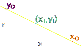
| Two-intercept equation |
$\frac{x}{x_∘}+\frac{y}{y_∘}=1, \medspace x_∘≠0 \land y_∘≠0$ |
Proof of Two-Intercept Equation
Use the coordinates for the intercepts in the slope of a line equation, which are interchangeable
$$m=\frac{0-y_∘}{x_∘-0}=\frac{y_∘-0}{0-x_∘}=-\frac{y_∘}{x_∘}$$
Substitute it into the slope-intercept equation
$$y=y_∘-\frac{y_∘}{x_∘}·x$$
Divide by $y_∘$ and isolate $1$
3.1.2 Systems of Linear Equations
Two Line Relations
Two equations that intersect will have the same $(x,y)$ coordinates and different slopes
| Parallel lines |
$m_1=m_2$ |
| Intercepting lines |
$m_1 \ne m_2$ |
| Perpendicular lines |
$m_1=-1/m_2$ |
Intersection Solves by Addition
Two equations may be added to each other. Like variables must be on the same side of the equation.
$$\begin{array}{r}
-2·x+9·y=5\\
\phantom{-}2·x-5·y=3\\
\overline{\phantom{-3·x+}4·y=8}\\
\end{array}$$
When one variable is solved, its value can be plugged into either of the equations to solve for the other variable. If the solution appears as
$0=n$, then the lines are parallel.
Intersection Solves by Isolation
Given two equations with different slopes
$$y=m_1·x+y_1\qquad y=m_2·x+y_2$$
To solve for $x$, set the equations equal to each other
$$m_1·x+y_1=m_2·x+y_2$$
Subtract $y_1$ and $m_2·x$
$$m_1·x-m_2·x=y_2-y_1$$
Factor
$$(m_1-m_2)·x=y_2-y_1$$
Isolate $x$
$$x=\frac{y_2-y_1}{m_1-m_2}$$
The value of $x$ can be plugged into either of the equations to solve for $y$. If the solution appears as $n/0$, then the lines are parallel.
3.1.3 Matrix Notation
A matrix can be used to display the
coefficients of linear expressions
$$
\begin{array}{c}
3·x+2·y \\
4·x-1·y
\end{array}
↔
\begin{bmatrix}
3 & \phantom{0}2 \\
4 & -1
\end{bmatrix}
$$
A joined matrix can be used to display the coefficients of
linear eqautions in the general form, with the constants in a separate column
$$
\begin{array}{c}
3·x+2·y=25 \\
4·x-1·y=\phantom{0}4
\end{array}
↔
\begin{bmatrix}
\begin{array}{cc|c}
3 & \phantom{-}2 & 25 \\
4 & -1 & \phantom{0}4
\end{array}
\end{bmatrix}
$$
Row Operations
A joined matrix representing linear equations allows for certain arithmetical operations on individual rows
1. Multiplication of a row
$$
\begin{array}{cc}
\\
2 & ·
\end{array}
\begin{bmatrix}
\begin{array}{cc|c}
3 & \phantom{-}2 & 25 \\
4 & -1 & \phantom{0}4
\end{array}
\end{bmatrix}
=
\begin{bmatrix}
\begin{array}{cc|c}
3 & \phantom{-}2 & 25 \\
8 & -2 & \phantom{0}8
\end{array}
\end{bmatrix}
$$
2. Addition of one row to another
$$
\begin{array}{c}
\text{R1} \\
\text{R2}
\end{array}
\begin{bmatrix}
\begin{array}{cc|c}
3 & \phantom{-}2 & 25 \\
8 & -2 & \phantom{0}8
\end{array}
\end{bmatrix}
$$
$$
\begin{array}{c}
\text{R1\phantom{+R2}} \\
\text{R1+R2}
\end{array}
\begin{bmatrix}
\begin{array}{cc|c}
\phantom{0}3 & 2 & 25 \\
11 & 0 & 33
\end{array}
\end{bmatrix}
$$
3. Switching rows
$$
\begin{bmatrix}
\begin{array}{cc|c}
11 & 0 & 33 \\
\phantom{0}3 & 2 & 25
\end{array}
\end{bmatrix}
$$
The aim is to create a matrix to display the values for $(1·x,1·y)$ in the column with constants. If this is unattainable, then the lines are parallel.
Example
To continue solving for the above, divide row 1 by 11
$$
\begin{bmatrix}
\begin{array}{cc|c}
1 & 0 & \phantom{0}3 \\
3 & 2 & 25
\end{array}
\end{bmatrix}
$$
Add row 1 multiplied by –3 to row 2
$$
\begin{bmatrix}
\begin{array}{cc|c}
1 & 0 & \phantom{0}3 \\
0 & 2 & 16
\end{array}
\end{bmatrix}
$$
Divide row 2 by 2
$$
\begin{bmatrix}
\begin{array}{cc|c}
1 & 0 & 3 \\
0 & 1 & 8
\end{array}
\end{bmatrix}
$$
The two equations intersect at $(x,y)=(3,8)$